>> 读入文本文档:readr 包
readr 的图形化用户界面 *
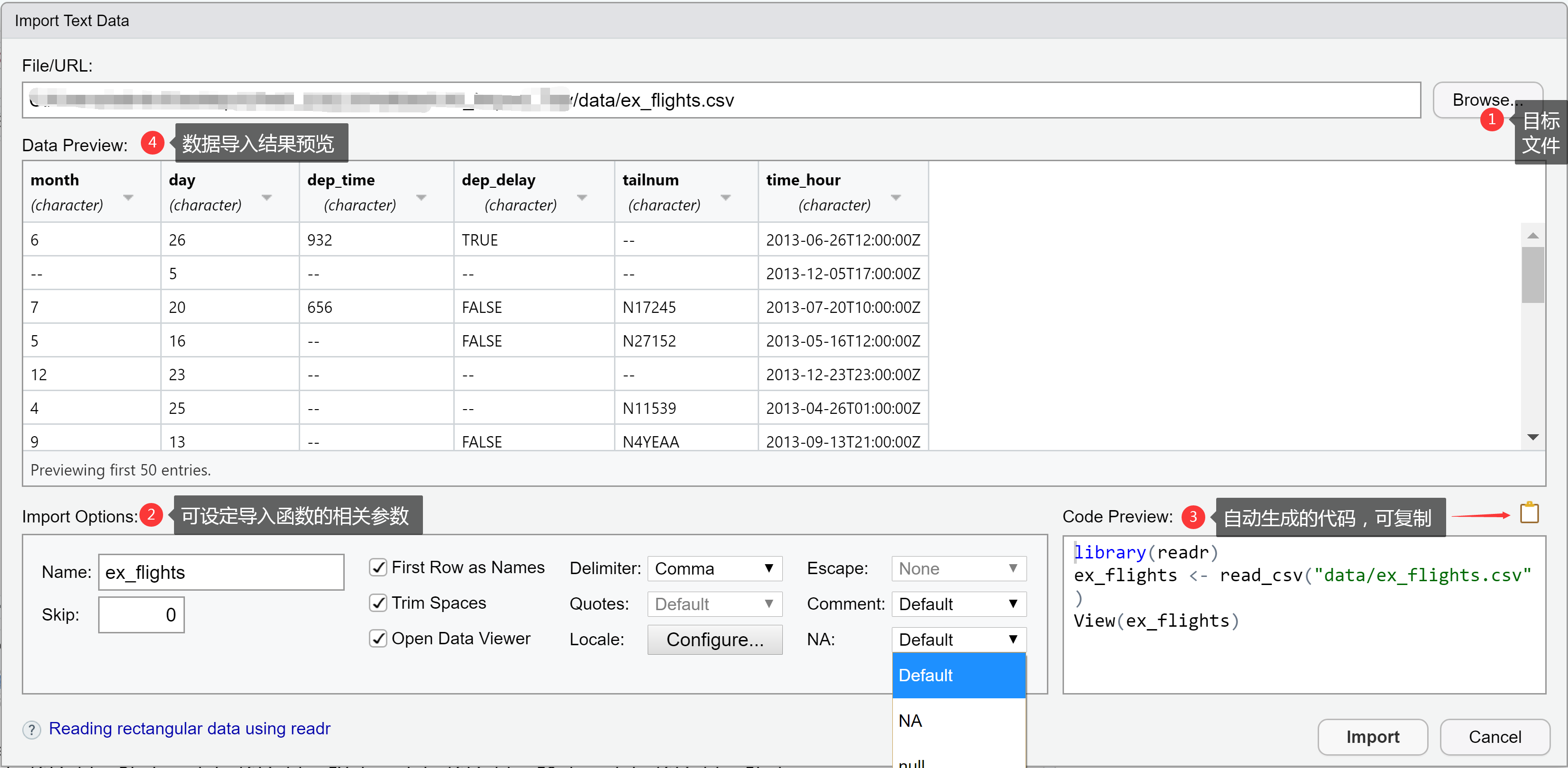
* RStudio 右上 Environment 标签页 > Import Dataset > From Text (readr) ...
>> 读入其它类型的数据
readr::read_rds():Rdata files (.rds)

{{: Read and Write Rectangular Text Data Quicklyvroom}} {{
{{readxl}}: excel files (.xls and .xlsx) <- take a 🧐 at it! {{
{{haven}}: SPSS, Stata, and SAS files {{
{{arrow}}: Apache Arrow
>> 读入其它类型的数据
readr::read_rds():Rdata files (.rds)
-
{{: Read and Write Rectangular Text Data Quicklyvroom}} - {{
readxl}}: excel files (.xls and .xlsx) <- take a 🧐 at it! - {{
haven}}: SPSS, Stata, and SAS files - {{
arrow}}: Apache Arrow
>> 读入其它类型的数据
readr::read_rds():Rdata files (.rds)
-
{{: Read and Write Rectangular Text Data Quicklyvroom}} - {{
readxl}}: excel files (.xls and .xlsx) <- take a 🧐 at it! - {{
haven}}: SPSS, Stata, and SAS files - {{
arrow}}: Apache Arrow
- {{其它}}: text、network、spatial、genome、image 等类型的数据
>> 齐整数据
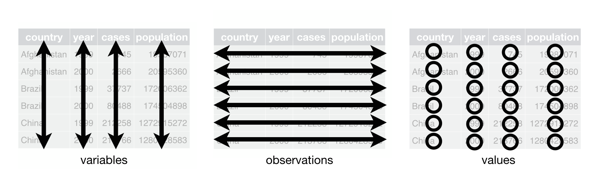
齐整数据的三个条件 📐
每列都是一个变量(Every column is a variable.)
每行都是一个观测(Every row is an observation.)
每格都是一个取值(Every cell is a single value.)
>> 齐整数据
齐整数据的好处 💪
☑ 齐整数据按照逻辑一致的方式存储数据,这让你更容易学习并掌握相关工具对数据进行处理
☑ “每列都是一个变量”及“每行都是一个观测”有助于发挥 R 语言向量化操作的优势
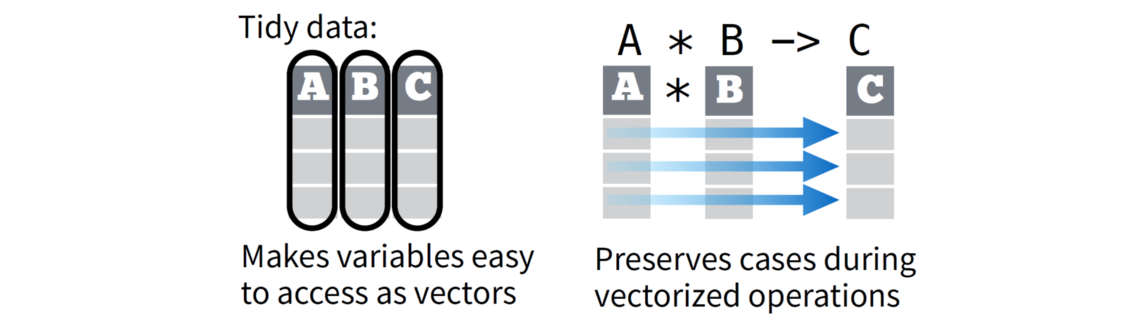
☑ tidyverse 中的 R 包(如 dplyr 等)在设计上要求输入数据为齐整数据
>> pivot_longer() 和 pivot_wider()
>> pivot_longer() 和 pivot_wider()
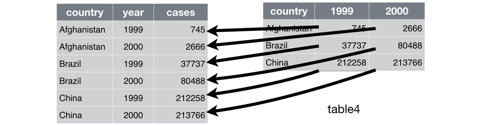
pivot_longer( data, cols, names_to = "name", names_prefix = NULL, names_sep = NULL, names_pattern = NULL, names_ptypes = NULL, names_transform = NULL, names_repair = "check_unique", values_to = "value", values_drop_na = FALSE, values_ptypes = NULL, values_transform = NULL, ...)>> pivot_longer() 和 pivot_wider()
pivot_longer( data, cols, names_to = "name", names_prefix = NULL, names_sep = NULL, names_pattern = NULL, names_ptypes = NULL, names_transform = NULL, names_repair = "check_unique", values_to = "value", values_drop_na = FALSE, values_ptypes = NULL, values_transform = NULL, ...)table4a %>% pivot_longer( cols = c(`1999`, `2000`), names_to = "year", values_to = "cases" )# table4b %>% ...#> # A tibble: 6 × 3#> country year cases#> <chr> <chr> <int>#> 1 Afghanistan 1999 745#> 2 Afghanistan 2000 2666#> 3 Brazil 1999 37737#> # … with 3 more rows>> pivot_longer() 和 pivot_wider()
>> pivot_longer() 和 pivot_wider()
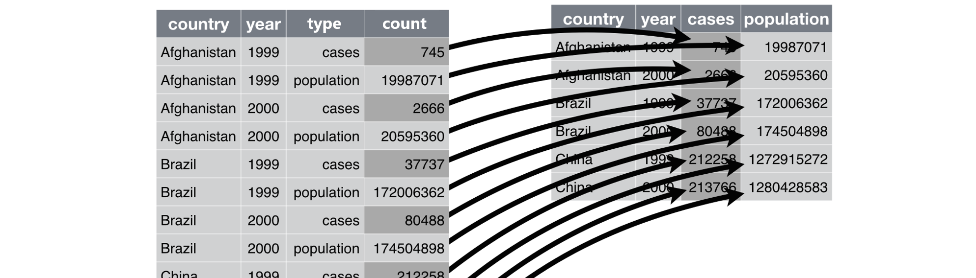
pivot_wider( data, id_cols = NULL, id_expand = FALSE, names_from = name, names_prefix = "", names_sep = "_", names_glue = NULL, names_sort = FALSE, names_vary = "fastest", names_expand = FALSE, names_repair = "check_unique", values_from = value, values_fill = NULL, values_fn = NULL, unused_fn = NULL, ...)>> pivot_longer() 和 pivot_wider()
pivot_wider( data, id_cols = NULL, id_expand = FALSE, names_from = name, names_prefix = "", names_sep = "_", names_glue = NULL, names_sort = FALSE, names_vary = "fastest", names_expand = FALSE, names_repair = "check_unique", values_from = value, values_fill = NULL, values_fn = NULL, unused_fn = NULL, ...)table2 %>% pivot_wider( names_from = type, values_from = count )#> # A tibble: 6 × 4#> country year cases population#> <chr> <int> <int> <int>#> 1 Afghanistan 1999 745 19987071#> 2 Afghanistan 2000 2666 20595360#> 3 Brazil 1999 37737 172006362#> # … with 3 more rows>> separate()、extract() 和 unite()
>> separate()、extract() 和 unite()
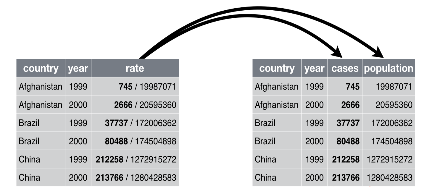
separate( data, col, into, sep = "[^[:alnum:]]+", remove = TRUE, convert = FALSE, extra = "warn", fill = "warn", ...)extract( data, col, into, regex = "([[:alnum:]]+)", remove = TRUE, convert = FALSE, ...)separate_rows(data, ..., sep, convert)>> separate()、extract() 和 unite()
separate( data, col, into, sep = "[^[:alnum:]]+", remove = TRUE, convert = FALSE, extra = "warn", fill = "warn", ...)extract( data, col, into, regex = "([[:alnum:]]+)", remove = TRUE, convert = FALSE, ...)separate_rows(data, ..., sep, convert)table3 %>% separate( rate, into = c("cases", "population"), convert = TRUE )#> # A tibble: 6 × 4#> country year cases population#> <chr> <int> <int> <int>#> 1 Afghanistan 1999 745 19987071#> 2 Afghanistan 2000 2666 20595360#> 3 Brazil 1999 37737 172006362#> # … with 3 more rows>> separate()、extract() 和 unite()
>> separate()、extract() 和 unite()
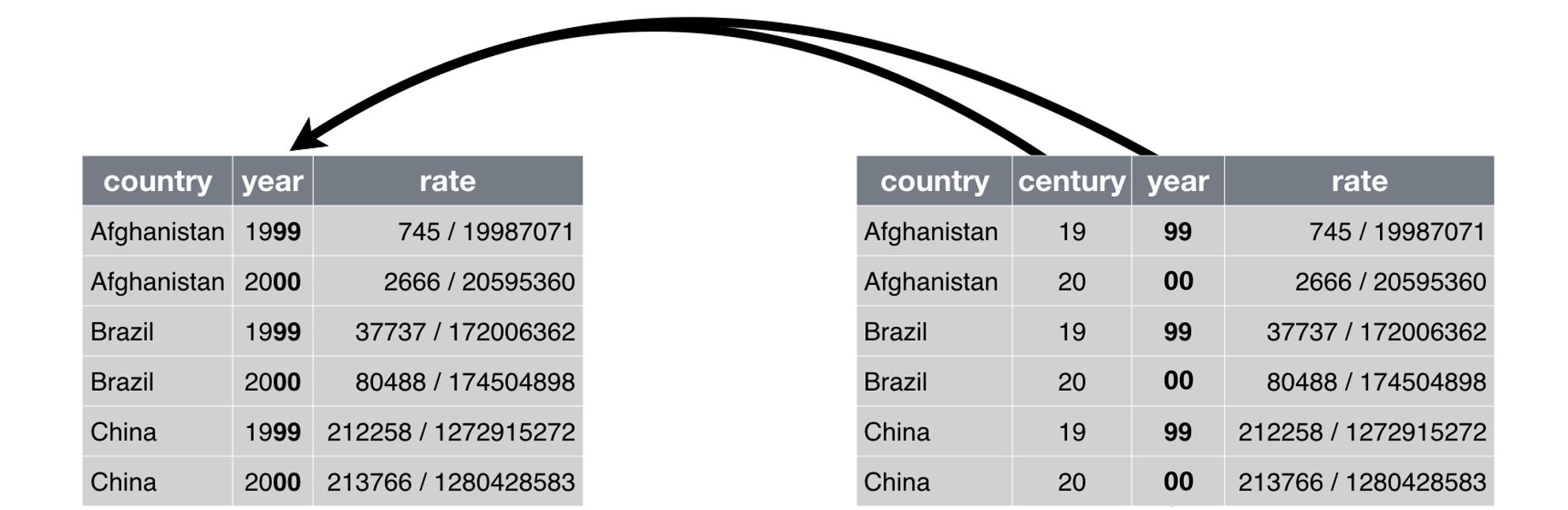
unite( data, col, ..., sep = "_", remove = TRUE, na.rm = FALSE)>> separate()、extract() 和 unite()
unite( data, col, ..., sep = "_", remove = TRUE, na.rm = FALSE)table5 %>% unite( col = "year", century, year, sep = "" )#> # A tibble: 6 × 3#> country year rate #> <chr> <chr> <chr> #> 1 Afghanistan 1999 745/19987071 #> 2 Afghanistan 2000 2666/20595360 #> 3 Brazil 1999 37737/172006362#> # … with 3 more rows>> unnest_* 和 hoist()
repurrrsive::gh_repos %>% View()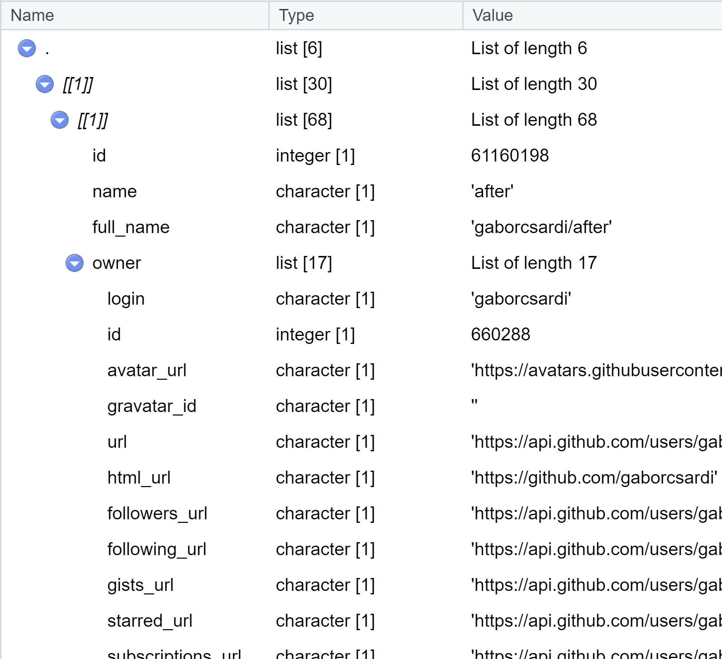
>> unnest_* 和 hoist()
repurrrsive::gh_repos %>% View()
(repos <- tibble(repo = repurrrsive::gh_repos))#> # A tibble: 6 × 1#> repo #> <list> #> 1 <list [30]>#> 2 <list [30]>#> 3 <list [30]>#> 4 <list [26]>#> 5 <list [30]>#> # … with 1 more row(repos <- repos %>% unnest_longer(repo))#> # A tibble: 176 × 1#> repo #> <list> #> 1 <named list [68]>#> 2 <named list [68]>#> 3 <named list [68]>#> 4 <named list [68]>#> 5 <named list [68]>#> # … with 171 more rows